September 9, 2019
Loan Default Data Wrangling
This rmarkdown document is an attempt to wrangle and fit a simple logistic regression model to Lending club loan dataset to predict the default rate of the loan (https://www.kaggle.com/wendykan/lending-club-loan-data). Other machine learning models can be easily fit to the dataset but I chose the simplest logistic regression to illustrate the entire process of wrangling data to productionizing the model. The dataset has been updated since I started working on this project so the some of the column names might not match. I can pass along the dataset I used in this project, but it is a relatively large file (431 MB).
I use dplyr package in this project to read and modify the dataset. plotly and ggplot2 will be used for some visualization. The goal is to create a simplified dataset, by removing NAs and variable which are irrelevant to the problem at hand, that is predicting the probabililty of loan defaults.
Load and view the dataset
df <- read_csv("C:/Users/Arun_Laptop/Desktop/DataScience/Loan_Default/loan.csv")
#df <- read_csv('loan.csv')An overview of all the columns and their types.
df %>%
glimpse()## Observations: 887,379
## Variables: 74
## $ id <dbl> 1077501, 1077430, 1077175, 1076863, 107...
## $ member_id <dbl> 1296599, 1314167, 1313524, 1277178, 131...
## $ loan_amnt <dbl> 5000, 2500, 2400, 10000, 3000, 5000, 70...
## $ funded_amnt <dbl> 5000, 2500, 2400, 10000, 3000, 5000, 70...
## $ funded_amnt_inv <dbl> 4975.00, 2500.00, 2400.00, 10000.00, 30...
## $ term <chr> "36 months", "60 months", "36 months", ...
## $ int_rate <dbl> 10.65, 15.27, 15.96, 13.49, 12.69, 7.90...
## $ installment <dbl> 162.87, 59.83, 84.33, 339.31, 67.79, 15...
## $ grade <chr> "B", "C", "C", "C", "B", "A", "C", "E",...
## $ sub_grade <chr> "B2", "C4", "C5", "C1", "B5", "A4", "C5...
## $ emp_title <chr> NA, "Ryder", NA, "AIR RESOURCES BOARD",...
## $ emp_length <chr> "10+ years", "< 1 year", "10+ years", "...
## $ home_ownership <chr> "RENT", "RENT", "RENT", "RENT", "RENT",...
## $ annual_inc <dbl> 24000.00, 30000.00, 12252.00, 49200.00,...
## $ verification_status <chr> "Verified", "Source Verified", "Not Ver...
## $ issue_d <chr> "Dec-2011", "Dec-2011", "Dec-2011", "De...
## $ loan_status <chr> "Fully Paid", "Charged Off", "Fully Pai...
## $ pymnt_plan <chr> "n", "n", "n", "n", "n", "n", "n", "n",...
## $ url <chr> "https://www.lendingclub.com/browse/loa...
## $ desc <chr> "Borrower added on 12/22/11 > I need to...
## $ purpose <chr> "credit_card", "car", "small_business",...
## $ title <chr> "Computer", "bike", "real estate busine...
## $ zip_code <chr> "860xx", "309xx", "606xx", "917xx", "97...
## $ addr_state <chr> "AZ", "GA", "IL", "CA", "OR", "AZ", "NC...
## $ dti <dbl> 27.65, 1.00, 8.72, 20.00, 17.94, 11.20,...
## $ delinq_2yrs <dbl> 0, 0, 0, 0, 0, 0, 0, 0, 0, 0, 0, 0, 0, ...
## $ earliest_cr_line <chr> "Jan-1985", "Apr-1999", "Nov-2001", "Fe...
## $ inq_last_6mths <dbl> 1, 5, 2, 1, 0, 3, 1, 2, 2, 0, 2, 0, 1, ...
## $ mths_since_last_delinq <dbl> NA, NA, NA, 35, 38, NA, NA, NA, NA, NA,...
## $ mths_since_last_record <dbl> NA, NA, NA, NA, NA, NA, NA, NA, NA, NA,...
## $ open_acc <dbl> 3, 3, 2, 10, 15, 9, 7, 4, 11, 2, 14, 12...
## $ pub_rec <dbl> 0, 0, 0, 0, 0, 0, 0, 0, 0, 0, 0, 0, 0, ...
## $ revol_bal <dbl> 13648, 1687, 2956, 5598, 27783, 7963, 1...
## $ revol_util <dbl> 83.70, 9.40, 98.50, 21.00, 53.90, 28.30...
## $ total_acc <dbl> 9, 4, 10, 37, 38, 12, 11, 4, 13, 3, 23,...
## $ initial_list_status <lgl> FALSE, FALSE, FALSE, FALSE, FALSE, FALS...
## $ out_prncp <dbl> 0.00, 0.00, 0.00, 0.00, 766.90, 0.00, 1...
## $ out_prncp_inv <dbl> 0.00, 0.00, 0.00, 0.00, 766.90, 0.00, 1...
## $ total_pymnt <dbl> 5861.071, 1008.710, 3003.654, 12226.302...
## $ total_pymnt_inv <dbl> 5831.78, 1008.71, 3003.65, 12226.30, 32...
## $ total_rec_prncp <dbl> 5000.00, 456.46, 2400.00, 10000.00, 223...
## $ total_rec_int <dbl> 861.07, 435.17, 603.65, 2209.33, 1009.0...
## $ total_rec_late_fee <dbl> 0.00, 0.00, 0.00, 16.97, 0.00, 0.00, 0....
## $ recoveries <dbl> 0.00, 117.08, 0.00, 0.00, 0.00, 0.00, 0...
## $ collection_recovery_fee <dbl> 0.0000, 1.1100, 0.0000, 0.0000, 0.0000,...
## $ last_pymnt_d <chr> "Jan-2015", "Apr-2013", "Jun-2014", "Ja...
## $ last_pymnt_amnt <dbl> 171.62, 119.66, 649.91, 357.48, 67.79, ...
## $ next_pymnt_d <chr> NA, NA, NA, NA, "Feb-2016", NA, "Feb-20...
## $ last_credit_pull_d <chr> "Jan-2016", "Sep-2013", "Jan-2016", "Ja...
## $ collections_12_mths_ex_med <dbl> 0, 0, 0, 0, 0, 0, 0, 0, 0, 0, 0, 0, 0, ...
## $ mths_since_last_major_derog <lgl> NA, NA, NA, NA, NA, NA, NA, NA, NA, NA,...
## $ policy_code <dbl> 1, 1, 1, 1, 1, 1, 1, 1, 1, 1, 1, 1, 1, ...
## $ application_type <chr> "INDIVIDUAL", "INDIVIDUAL", "INDIVIDUAL...
## $ annual_inc_joint <lgl> NA, NA, NA, NA, NA, NA, NA, NA, NA, NA,...
## $ dti_joint <lgl> NA, NA, NA, NA, NA, NA, NA, NA, NA, NA,...
## $ verification_status_joint <lgl> NA, NA, NA, NA, NA, NA, NA, NA, NA, NA,...
## $ acc_now_delinq <dbl> 0, 0, 0, 0, 0, 0, 0, 0, 0, 0, 0, 0, 0, ...
## $ tot_coll_amt <lgl> NA, NA, NA, NA, NA, NA, NA, NA, NA, NA,...
## $ tot_cur_bal <lgl> NA, NA, NA, NA, NA, NA, NA, NA, NA, NA,...
## $ open_acc_6m <lgl> NA, NA, NA, NA, NA, NA, NA, NA, NA, NA,...
## $ open_il_6m <lgl> NA, NA, NA, NA, NA, NA, NA, NA, NA, NA,...
## $ open_il_12m <lgl> NA, NA, NA, NA, NA, NA, NA, NA, NA, NA,...
## $ open_il_24m <lgl> NA, NA, NA, NA, NA, NA, NA, NA, NA, NA,...
## $ mths_since_rcnt_il <lgl> NA, NA, NA, NA, NA, NA, NA, NA, NA, NA,...
## $ total_bal_il <lgl> NA, NA, NA, NA, NA, NA, NA, NA, NA, NA,...
## $ il_util <lgl> NA, NA, NA, NA, NA, NA, NA, NA, NA, NA,...
## $ open_rv_12m <lgl> NA, NA, NA, NA, NA, NA, NA, NA, NA, NA,...
## $ open_rv_24m <lgl> NA, NA, NA, NA, NA, NA, NA, NA, NA, NA,...
## $ max_bal_bc <lgl> NA, NA, NA, NA, NA, NA, NA, NA, NA, NA,...
## $ all_util <lgl> NA, NA, NA, NA, NA, NA, NA, NA, NA, NA,...
## $ total_rev_hi_lim <lgl> NA, NA, NA, NA, NA, NA, NA, NA, NA, NA,...
## $ inq_fi <lgl> NA, NA, NA, NA, NA, NA, NA, NA, NA, NA,...
## $ total_cu_tl <lgl> NA, NA, NA, NA, NA, NA, NA, NA, NA, NA,...
## $ inq_last_12m <lgl> NA, NA, NA, NA, NA, NA, NA, NA, NA, NA,...Visualizing the NAs in the dataset
vect_NA <- apply(df,2,lenNA)
vect_NA = vect_NA/length(df[,1])p <- plot_ly(
x = names(vect_NA),
y = vect_NA,
name = "NA Bar Chart",
type = 'bar'
) %>%
layout(title = 'Columns with NA',yaxis = list(title = '% NA',tickformat = '%'))
pRemove NAs
Removing all NAs and assigning the results to a new data frame
df_NA <- df %>%
select_if(function(x) any(is.na(x))) %>%
summarise_each(funs(sum(is.na(.)))) %>%
select_if(function(x) any(x>400000))
df_NA %>% glimpse()## Observations: 1
## Variables: 25
## $ desc <int> 761597
## $ mths_since_last_delinq <int> 454312
## $ mths_since_last_record <int> 750326
## $ initial_list_status <int> 430531
## $ mths_since_last_major_derog <int> 887379
## $ annual_inc_joint <int> 887379
## $ dti_joint <int> 887379
## $ verification_status_joint <int> 887379
## $ tot_coll_amt <int> 887379
## $ tot_cur_bal <int> 887379
## $ open_acc_6m <int> 887379
## $ open_il_6m <int> 887379
## $ open_il_12m <int> 887379
## $ open_il_24m <int> 887379
## $ mths_since_rcnt_il <int> 887379
## $ total_bal_il <int> 887379
## $ il_util <int> 887379
## $ open_rv_12m <int> 887379
## $ open_rv_24m <int> 887379
## $ max_bal_bc <int> 887379
## $ all_util <int> 887379
## $ total_rev_hi_lim <int> 887379
## $ inq_fi <int> 887379
## $ total_cu_tl <int> 887379
## $ inq_last_12m <int> 887379df_new <- df %>%
select(-c(colnames(df_NA)))Plotting Geographical Location of Loans
Loan aggregation by state. Simple group by statement is used to aggregate data at the State level. Things like number of loan requests, total loan amount, mean loan amount are plotted on a US choropleth plot with state boundaries.
total_loan_req_by_state <- df_new %>% group_by(addr_state) %>%
summarize(total_reqs = n())
total_loan_by_state <- df_new %>% group_by(addr_state) %>%
summarise(total_loan = sum(loan_amnt))
mean_loan_by_state <- df_new %>% group_by(addr_state) %>%
summarise(mean_loan = round(mean(loan_amnt),3))
median_loan_by_state <- df_new %>% group_by(addr_state) %>%
summarize(median_loan = median(loan_amnt))California has the highest number of loan requests of any state. This could be related to the number of people living in California.Tranforming the plot to a per capita level will reveal whether people in California have a greater tendency to request for a loan compared to other states.
#loan_agg_state$TotalLoanAmount <- loan_agg_state$TotalLoanAmount
l <- list(color = toRGB("white"), width = 2)
g <- list(
scope = 'usa',
projection = list(type = 'albers usa'),
showlakes = TRUE,
lakecolor = toRGB('white')
)
p1 <- plot_geo(total_loan_req_by_state, locationmode = 'USA-states') %>%
add_trace(z = ~total_reqs,locations = ~addr_state,
color = ~total_reqs,colors=colorRamp(c('blue','green','yellow','red')))%>%
colorbar(title = "Number of Loan Requests") %>%
layout(
title = 'Total Number of Loan Requests from each US state',
geo = g
)
p1p2 <- plot_geo(total_loan_by_state, locationmode = 'USA-states') %>%
add_trace(z = ~total_loan,locations = ~addr_state,
color = ~total_loan,colors=colorRamp(c('blue','green','yellow','red')))%>%
colorbar(title = "Total Loan in USD") %>%
layout(
title = 'Total Loan in USD by State',
geo = g
)
p2p3 <- plot_geo(mean_loan_by_state, locationmode = 'USA-states') %>%
add_trace(z = ~round(mean_loan,3),locations = ~addr_state,
color = ~round(mean_loan,3),colors=colorRamp(c('blue','green','yellow','red')))%>%
colorbar(title = "Mean Loan in USD") %>%
layout(
title = 'Mean Loan in USD by State',
geo = g
)
p3df_new %>%
select(loan_amnt,addr_state) %>%
plot_ly(y=~loan_amnt,color=~addr_state,type='box',colors = 'Set1') %>%
layout(title = '<b>Loan Amount Distribution by State</b>',
yaxis = list(title = '<b>Loan Amnt in USD</b>'))p4 <- plot_geo(median_loan_by_state, locationmode = 'USA-states') %>%
add_trace(z = ~median_loan,locations = ~addr_state,
color = ~median_loan,colors=colorRamp(c('blue','green','yellow','red')))%>%
colorbar(title = "Median Loan in USD") %>%
layout(
title = 'Median Loan in USD by State',
geo = g
)
p4Another parameter which can be looked at is the number of loans defaulted in each state. The loan default variable has many categories. To keep things simple, the number of categories is reduced to 2 - for binary classification. The two levels are not defaulted and defaulted.
df_new <- df_new %>%
mutate(loan_status = ifelse((loan_status !='Fully Paid' & loan_status !='Issued' & loan_status != 'Current'),'Default','Good'))Creating a new dataframe by grouping loan defaults by state. The simple group by and summarise pipes
default_by_state <- df_new %>%
group_by(addr_state,loan_status) %>%
summarise(count = n())
default_by_state## # A tibble: 102 x 3
## # Groups: addr_state [51]
## addr_state loan_status count
## <chr> <chr> <int>
## 1 AK Default 155
## 2 AK Good 2050
## 3 AL Default 1017
## 4 AL Good 10183
## 5 AR Default 516
## 6 AR Good 6124
## 7 AZ Default 1614
## 8 AZ Good 18798
## 9 CA Default 10741
## 10 CA Good 118776
## # ... with 92 more rowsp5 <- plot_geo(default_by_state %>%
filter(loan_status =='Default') %>%
mutate(count = as.double(count)),
locationmode = 'USA-states') %>%
add_trace(z = ~count,
locations = ~addr_state,
color = ~count,
colors=colorRamp(c('blue','green','yellow','red'))
)%>%
colorbar(title = "Number of Loan Defaults") %>%
layout(
title = 'Number of Loan Defaults',
geo = g
)
p5default_percent_by_state <- (default_by_state %>%
filter(loan_status == 'Default')) %>%
inner_join(default_by_state %>%
group_by(addr_state) %>%
summarise(total = sum(count))
) %>%
mutate(percent_default = round(100*count/total,2))g1 <- list(
scope = 'usa',
projection = list(type = 'albers usa'),
showlakes = TRUE,
tickformat = "%",
lakecolor = toRGB('white')
)
p6 <- plot_geo(default_percent_by_state, locationmode = 'USA-states') %>%
add_trace(z = ~percent_default,
locations = ~addr_state,
color = ~percent_default,
colors=colorRamp(c('blue','green','yellow','red'))
)%>%
colorbar(title = "Total % of Loan Defaults") %>%
layout(
title = 'Total Number of Loan Default Percentage by State',
geo = g1
)
p6The above plot shows that there are 2 states with high default rates, Iowa and Idaho. Looking into the dataset, it is clear that there were very few loans from both the states and the reason they are outliers.
default_by_state %>%
filter(addr_state == 'IA' | addr_state == 'ID') ## # A tibble: 4 x 3
## # Groups: addr_state [2]
## addr_state loan_status count
## <chr> <chr> <int>
## 1 IA Default 8
## 2 IA Good 6
## 3 ID Default 4
## 4 ID Good 8Cleanup of the dataset & further EDA
The dataset after removing majority NA columns has 49 variables. Further exploration is done to see whether there are any correlated variables which can be removed. The metadata which is avaialble on the Kaggle webpage is imported to understand the description of some of the variables which remain after the NA removal
metadata <- read_csv("LCDataDictionary.csv") %>%
rename(col_names = LoanStatNew)
df_colnames <- data.frame(col_names = as.character(df_new %>% colnames()))
metadata <- metadata %>%
inner_join(df_colnames, by = 'col_names')
metadata %>% kable() %>%
kable_styling(bootstrap_options = c("striped", "hover"),position = 'center') %>%
scroll_box(width = "100%", height = "200px")| col_names | Description |
|---|---|
| addr_state | The state provided by the borrower in the loan application |
| annual_inc | The self-reported annual income provided by the borrower during registration. |
| application_type | Indicates whether the loan is an individual application or a joint application with two co-borrowers |
| collection_recovery_fee | post charge off collection fee |
| collections_12_mths_ex_med | Number of collections in 12 months excluding medical collections |
| delinq_2yrs | The number of 30+ days past-due incidences of delinquency in the borrower’s credit file for the past 2 years |
| dti | A ratio calculated using the borrower’s total monthly debt payments on the total debt obligations, excluding mortgage and the requested LC loan, divided by the borrower’s self-reported monthly income. |
| earliest_cr_line | The month the borrower’s earliest reported credit line was opened |
| emp_length | Employment length in years. Possible values are between 0 and 10 where 0 means less than one year and 10 means ten or more years. |
| emp_title | The job title supplied by the Borrower when applying for the loan.* |
| funded_amnt | The total amount committed to that loan at that point in time. |
| funded_amnt_inv | The total amount committed by investors for that loan at that point in time. |
| grade | LC assigned loan grade |
| home_ownership | The home ownership status provided by the borrower during registration. Our values are: RENT, OWN, MORTGAGE, OTHER. |
| id | A unique LC assigned ID for the loan listing. |
| inq_last_6mths | The number of inquiries in past 6 months (excluding auto and mortgage inquiries) |
| installment | The monthly payment owed by the borrower if the loan originates. |
| int_rate | Interest Rate on the loan |
| issue_d | The month which the loan was funded |
| last_credit_pull_d | The most recent month LC pulled credit for this loan |
| last_pymnt_amnt | Last total payment amount received |
| last_pymnt_d | Last month payment was received |
| loan_amnt | The listed amount of the loan applied for by the borrower. If at some point in time, the credit department reduces the loan amount, then it will be reflected in this value. |
| loan_status | Current status of the loan |
| member_id | A unique LC assigned Id for the borrower member. |
| next_pymnt_d | Next scheduled payment date |
| open_acc | The number of open credit lines in the borrower’s credit file. |
| out_prncp | Remaining outstanding principal for total amount funded |
| out_prncp_inv | Remaining outstanding principal for portion of total amount funded by investors |
| policy_code | publicly available policy_code=1 new products not publicly available policy_code=2 |
| pub_rec | Number of derogatory public records |
| purpose | A category provided by the borrower for the loan request. |
| pymnt_plan | Indicates if a payment plan has been put in place for the loan |
| recoveries | post charge off gross recovery |
| revol_bal | Total credit revolving balance |
| revol_util | Revolving line utilization rate, or the amount of credit the borrower is using relative to all available revolving credit. |
| sub_grade | LC assigned loan subgrade |
| term | The number of payments on the loan. Values are in months and can be either 36 or 60. |
| title | The loan title provided by the borrower |
| total_acc | The total number of credit lines currently in the borrower’s credit file |
| total_pymnt | Payments received to date for total amount funded |
| total_pymnt_inv | Payments received to date for portion of total amount funded by investors |
| total_rec_int | Interest received to date |
| total_rec_late_fee | Late fees received to date |
| total_rec_prncp | Principal received to date |
| url | URL for the LC page with listing data. |
| zip_code | The first 3 numbers of the zip code provided by the borrower in the loan application. |
| acc_now_delinq | The number of accounts on which the borrower is now delinquent. |
The following columns are eliminated as they are not suitable for a classification model fitting and don’t have any predictive power. Reasons are given below
#
# head(df_new$earliest_cr_line)
# head(df_new$last_pymnt_d)
# head(df_new$next_pymnt_d)
#
# table(df_new$sub_grade)
# #ggplot(df_new)+geom_point(aes(x = out_prncp_inv,y=out_prncp))
#
# ggplot(df_new) + geom_histogram(aes( pub_rec))
#
# table(df_new$pub_rec)
# ggplot(df_new)+geom_point(aes(x = total_rec_prncp,y=total_pymnt))
df_new <- df_new %>%
select(-c(id,# A unique LC assigned ID for the loan listing.
member_id,# A unique LC assigned Id for the borrower member.
url,# URL for the LC page with listing data.
zip_code,# The first 3 numbers of the zip code provided by the borrower in the loan application.
addr_state, #The state provided by the borrower in the loan application
emp_title, #The job title supplied by the Borrower when applying for the loan
title, #The loan title provided by the borrower
policy_code, #publicly available policy_code=1\nnew products not publicly available policy_code=2. Just a single value of one
pymnt_plan,#Indicates if a payment plan has been put in place for the loan.
acc_now_delinq, #The number of accounts on which the borrower is now delinquent.. Mostly zeros
collections_12_mths_ex_med,#Number of collections in 12 months excluding medical collections. Mostly zeros
collection_recovery_fee, #Mostly zeros
#delinq_2yrs, #Mostly zeros
recoveries,#mostly zeros
out_prncp_inv, #Highly correlated with out_prncp
total_pymnt_inv, #Highly correlated with total_pymnt
total_rec_prncp,#Highly correlated with total_pymnt
application_type, #Majoirty of the factor is a single variable
total_rec_late_fee,# Mostly zero
earliest_cr_line, # A month & year without any referene,
last_pymnt_d, #A single date again without reference
next_pymnt_d, # A single date without reference and many NAs
funded_amnt,# Highly correlated with loan amount
funded_amnt_inv, #Highly correlated with laon amount
sub_grade #categorical variable with many levels without much explanation of what these levels represent
)
)The numher of columns reduced from 74 to 25 after the elimination of irrelavent variables
df_new %>% glimpse()## Observations: 887,379
## Variables: 25
## $ loan_amnt <dbl> 5000, 2500, 2400, 10000, 3000, 5000, 7000, 3000...
## $ term <chr> "36 months", "60 months", "36 months", "36 mont...
## $ int_rate <dbl> 10.65, 15.27, 15.96, 13.49, 12.69, 7.90, 15.96,...
## $ installment <dbl> 162.87, 59.83, 84.33, 339.31, 67.79, 156.46, 17...
## $ grade <chr> "B", "C", "C", "C", "B", "A", "C", "E", "F", "B...
## $ emp_length <chr> "10+ years", "< 1 year", "10+ years", "10+ year...
## $ home_ownership <chr> "RENT", "RENT", "RENT", "RENT", "RENT", "RENT",...
## $ annual_inc <dbl> 24000.00, 30000.00, 12252.00, 49200.00, 80000.0...
## $ verification_status <chr> "Verified", "Source Verified", "Not Verified", ...
## $ issue_d <chr> "Dec-2011", "Dec-2011", "Dec-2011", "Dec-2011",...
## $ loan_status <chr> "Good", "Default", "Good", "Good", "Good", "Goo...
## $ purpose <chr> "credit_card", "car", "small_business", "other"...
## $ dti <dbl> 27.65, 1.00, 8.72, 20.00, 17.94, 11.20, 23.51, ...
## $ delinq_2yrs <dbl> 0, 0, 0, 0, 0, 0, 0, 0, 0, 0, 0, 0, 0, 0, 0, 0,...
## $ inq_last_6mths <dbl> 1, 5, 2, 1, 0, 3, 1, 2, 2, 0, 2, 0, 1, 2, 2, 1,...
## $ open_acc <dbl> 3, 3, 2, 10, 15, 9, 7, 4, 11, 2, 14, 12, 4, 11,...
## $ pub_rec <dbl> 0, 0, 0, 0, 0, 0, 0, 0, 0, 0, 0, 0, 0, 0, 0, 0,...
## $ revol_bal <dbl> 13648, 1687, 2956, 5598, 27783, 7963, 17726, 82...
## $ revol_util <dbl> 83.70, 9.40, 98.50, 21.00, 53.90, 28.30, 85.60,...
## $ total_acc <dbl> 9, 4, 10, 37, 38, 12, 11, 4, 13, 3, 23, 34, 9, ...
## $ out_prncp <dbl> 0.00, 0.00, 0.00, 0.00, 766.90, 0.00, 1889.15, ...
## $ total_pymnt <dbl> 5861.071, 1008.710, 3003.654, 12226.302, 3242.1...
## $ total_rec_int <dbl> 861.07, 435.17, 603.65, 2209.33, 1009.07, 631.3...
## $ last_pymnt_amnt <dbl> 171.62, 119.66, 649.91, 357.48, 67.79, 161.03, ...
## $ last_credit_pull_d <chr> "Jan-2016", "Sep-2013", "Jan-2016", "Jan-2015",...Creation of a new variable - Days elasped after issuance of loan to first credit inquiry. This variable might have some predictive value compared to just plain date variables.
df_new <- df_new %>%
mutate(last_credit_pull_d = convert_date(last_credit_pull_d),
issue_d = convert_date(issue_d),
score_days_interval = last_credit_pull_d - issue_d)Reduction of home ownership categorical variable to fewer levels
df_new %>% select(home_ownership) %>% unique()## # A tibble: 6 x 1
## home_ownership
## <chr>
## 1 RENT
## 2 OWN
## 3 MORTGAGE
## 4 OTHER
## 5 NONE
## 6 ANYTo simplify the analysis OTHER, NONE and ANY Levels were removed.
df_new <- df_new %>%
filter(home_ownership!='NONE' &
home_ownership!='ANY' &
home_ownership!='OTHER')Conversion of all the character variables into factors
cls <- sapply(df_new,class) # Obtain classes of all the variables in a vector
#cls
df_new <- df_new %>%
select(which(cls=="character")) %>%
mutate_all(as.factor) %>%
mutate(id = row_number()) %>%
inner_join(df_new %>%
select(which(cls!="character")) %>%
mutate(id=row_number()), by='id') %>%
drop_na()
df_new %>% glimpse()## Observations: 886,596
## Variables: 27
## $ term <fct> 36 months, 60 months, 36 months, 36 months, 60 ...
## $ grade <fct> B, C, C, C, B, A, C, E, F, B, C, B, C, B, B, D,...
## $ emp_length <fct> 10+ years, < 1 year, 10+ years, 10+ years, 1 ye...
## $ home_ownership <fct> RENT, RENT, RENT, RENT, RENT, RENT, RENT, RENT,...
## $ verification_status <fct> Verified, Source Verified, Not Verified, Source...
## $ loan_status <fct> Good, Default, Good, Good, Good, Good, Good, Go...
## $ purpose <fct> credit_card, car, small_business, other, other,...
## $ id <int> 1, 2, 3, 4, 5, 6, 7, 8, 9, 10, 11, 12, 13, 14, ...
## $ loan_amnt <dbl> 5000, 2500, 2400, 10000, 3000, 5000, 7000, 3000...
## $ int_rate <dbl> 10.65, 15.27, 15.96, 13.49, 12.69, 7.90, 15.96,...
## $ installment <dbl> 162.87, 59.83, 84.33, 339.31, 67.79, 156.46, 17...
## $ annual_inc <dbl> 24000.00, 30000.00, 12252.00, 49200.00, 80000.0...
## $ issue_d <dbl> 15309, 15309, 15309, 15309, 15309, 15309, 15309...
## $ dti <dbl> 27.65, 1.00, 8.72, 20.00, 17.94, 11.20, 23.51, ...
## $ delinq_2yrs <dbl> 0, 0, 0, 0, 0, 0, 0, 0, 0, 0, 0, 0, 0, 0, 0, 0,...
## $ inq_last_6mths <dbl> 1, 5, 2, 1, 0, 3, 1, 2, 2, 0, 2, 0, 1, 2, 2, 1,...
## $ open_acc <dbl> 3, 3, 2, 10, 15, 9, 7, 4, 11, 2, 14, 12, 4, 11,...
## $ pub_rec <dbl> 0, 0, 0, 0, 0, 0, 0, 0, 0, 0, 0, 0, 0, 0, 0, 0,...
## $ revol_bal <dbl> 13648, 1687, 2956, 5598, 27783, 7963, 17726, 82...
## $ revol_util <dbl> 83.70, 9.40, 98.50, 21.00, 53.90, 28.30, 85.60,...
## $ total_acc <dbl> 9, 4, 10, 37, 38, 12, 11, 4, 13, 3, 23, 34, 9, ...
## $ out_prncp <dbl> 0.00, 0.00, 0.00, 0.00, 766.90, 0.00, 1889.15, ...
## $ total_pymnt <dbl> 5861.071, 1008.710, 3003.654, 12226.302, 3242.1...
## $ total_rec_int <dbl> 861.07, 435.17, 603.65, 2209.33, 1009.07, 631.3...
## $ last_pymnt_amnt <dbl> 171.62, 119.66, 649.91, 357.48, 67.79, 161.03, ...
## $ last_credit_pull_d <dbl> 16801, 15949, 16801, 16436, 16801, 16679, 16801...
## $ score_days_interval <dbl> 1492, 640, 1492, 1127, 1492, 1370, 1492, 1096, ...Removing date variables
df_new <- df_new %>%
select(-c(issue_d,
last_credit_pull_d))The kable package offers a way to view tables in a nice html format. Below is an attempt to display first 15 rows of the dataset as a html table
df_new %>%
head(10) %>%
kable() %>%
kable_styling(bootstrap_options = c("striped", "hover"),position = "center") %>%
scroll_box(width = "100%", height = "100%")| term | grade | emp_length | home_ownership | verification_status | loan_status | purpose | id | loan_amnt | int_rate | installment | annual_inc | dti | delinq_2yrs | inq_last_6mths | open_acc | pub_rec | revol_bal | revol_util | total_acc | out_prncp | total_pymnt | total_rec_int | last_pymnt_amnt | score_days_interval |
|---|---|---|---|---|---|---|---|---|---|---|---|---|---|---|---|---|---|---|---|---|---|---|---|---|
| 36 months | B | 10+ years | RENT | Verified | Good | credit_card | 1 | 5000 | 10.65 | 162.87 | 24000 | 27.65 | 0 | 1 | 3 | 0 | 13648 | 83.7 | 9 | 0.00 | 5861.071 | 861.07 | 171.62 | 1492 |
| 60 months | C | < 1 year | RENT | Source Verified | Default | car | 2 | 2500 | 15.27 | 59.83 | 30000 | 1.00 | 0 | 5 | 3 | 0 | 1687 | 9.4 | 4 | 0.00 | 1008.710 | 435.17 | 119.66 | 640 |
| 36 months | C | 10+ years | RENT | Not Verified | Good | small_business | 3 | 2400 | 15.96 | 84.33 | 12252 | 8.72 | 0 | 2 | 2 | 0 | 2956 | 98.5 | 10 | 0.00 | 3003.654 | 603.65 | 649.91 | 1492 |
| 36 months | C | 10+ years | RENT | Source Verified | Good | other | 4 | 10000 | 13.49 | 339.31 | 49200 | 20.00 | 0 | 1 | 10 | 0 | 5598 | 21.0 | 37 | 0.00 | 12226.302 | 2209.33 | 357.48 | 1127 |
| 60 months | B | 1 year | RENT | Source Verified | Good | other | 5 | 3000 | 12.69 | 67.79 | 80000 | 17.94 | 0 | 0 | 15 | 0 | 27783 | 53.9 | 38 | 766.90 | 3242.170 | 1009.07 | 67.79 | 1492 |
| 36 months | A | 3 years | RENT | Source Verified | Good | wedding | 6 | 5000 | 7.90 | 156.46 | 36000 | 11.20 | 0 | 3 | 9 | 0 | 7963 | 28.3 | 12 | 0.00 | 5631.378 | 631.38 | 161.03 | 1370 |
| 60 months | C | 8 years | RENT | Not Verified | Good | debt_consolidation | 7 | 7000 | 15.96 | 170.08 | 47004 | 23.51 | 0 | 1 | 7 | 0 | 17726 | 85.6 | 11 | 1889.15 | 8136.840 | 3025.99 | 170.08 | 1492 |
| 36 months | E | 9 years | RENT | Source Verified | Good | car | 8 | 3000 | 18.64 | 109.43 | 48000 | 5.35 | 0 | 2 | 4 | 0 | 8221 | 87.5 | 4 | 0.00 | 3938.144 | 938.14 | 111.34 | 1096 |
| 60 months | F | 4 years | OWN | Source Verified | Default | small_business | 9 | 5600 | 21.28 | 152.39 | 40000 | 5.55 | 0 | 2 | 11 | 0 | 5210 | 32.6 | 13 | 0.00 | 646.020 | 294.94 | 152.39 | 244 |
| 60 months | B | < 1 year | RENT | Verified | Default | other | 10 | 5375 | 12.69 | 121.45 | 15000 | 18.08 | 0 | 0 | 2 | 0 | 9279 | 36.5 | 3 | 0.00 | 1476.190 | 533.42 | 121.45 | 456 |
Save the reduced dataset in a RDS file for later use. This is a binary file format and hence is smaller in size on disk and also can be read faster compared to a traditional CSV file. There are 2 different formats. One is the native .RDS file and other is, feather file format which can also be read into Python.
loan_cleaned <- saveRDS(df_new,file = "loan_cleaned_RMD.rds")Feather file format
library(feather)
write_feather(df_new, "loan_cleaned.feather")Further EDA on the reduced dataset
The purpose of a predictive model is to establish correlation between features and the response variable. In a binary classification problem explanatory variables which provide class bifurcation visually, have good to excellent predictive power. The purpose of this section to perform simple visual analysis to explore the dataset further. The first variable is the Interest Rate Percent with loan_status being the response variable with 2 levels - “Default” and “Good”. The boxplot clearly shows that the there could be statistically significant difference between the distributions of Interest Rate % grouped by loan_status. Hence Interest Rate % could be used as good predictor variable. ggplot2 is used for visualization.
ggplot(df_new,aes(y=int_rate,fill=loan_status)) +
geom_boxplot() +
labs(y="Interest Rate %",
title = "Interest Rate %")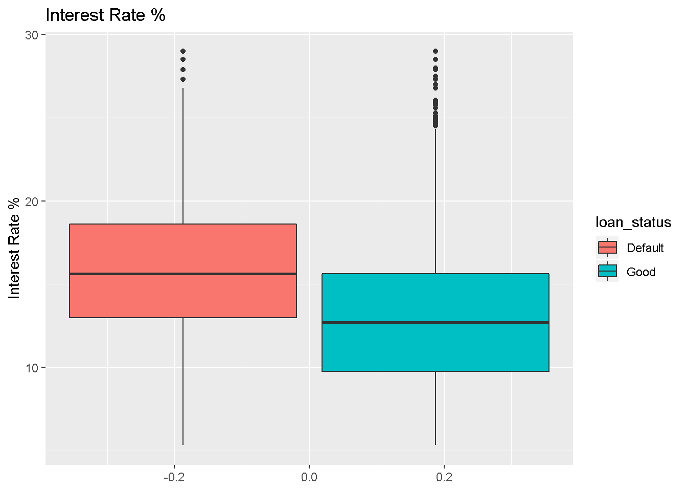
Figure 1: Boxplot of Interest Rate
Similar visualization is performed with few other variables. The number of days elasped variable also appears to be statistically significant indicator of Loan Default. (doesn’t necessary indicate practical significance)
ggplot(df_new,aes(y=score_days_interval,fill=loan_status))+
geom_boxplot() +
labs(y = "Days Elapsed",
title="Number of Days elasped between loan issuance and first credit pull")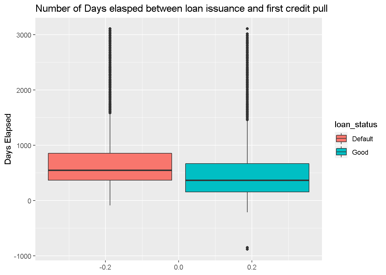
Loan Amount Requested variable by itself doesn’t appear to show class boundary separation.
ggplot(df_new,aes(y=loan_amnt,fill=loan_status))+
geom_boxplot() +
labs(y='Loan Amount ($)',title = "Loan Amount Requested")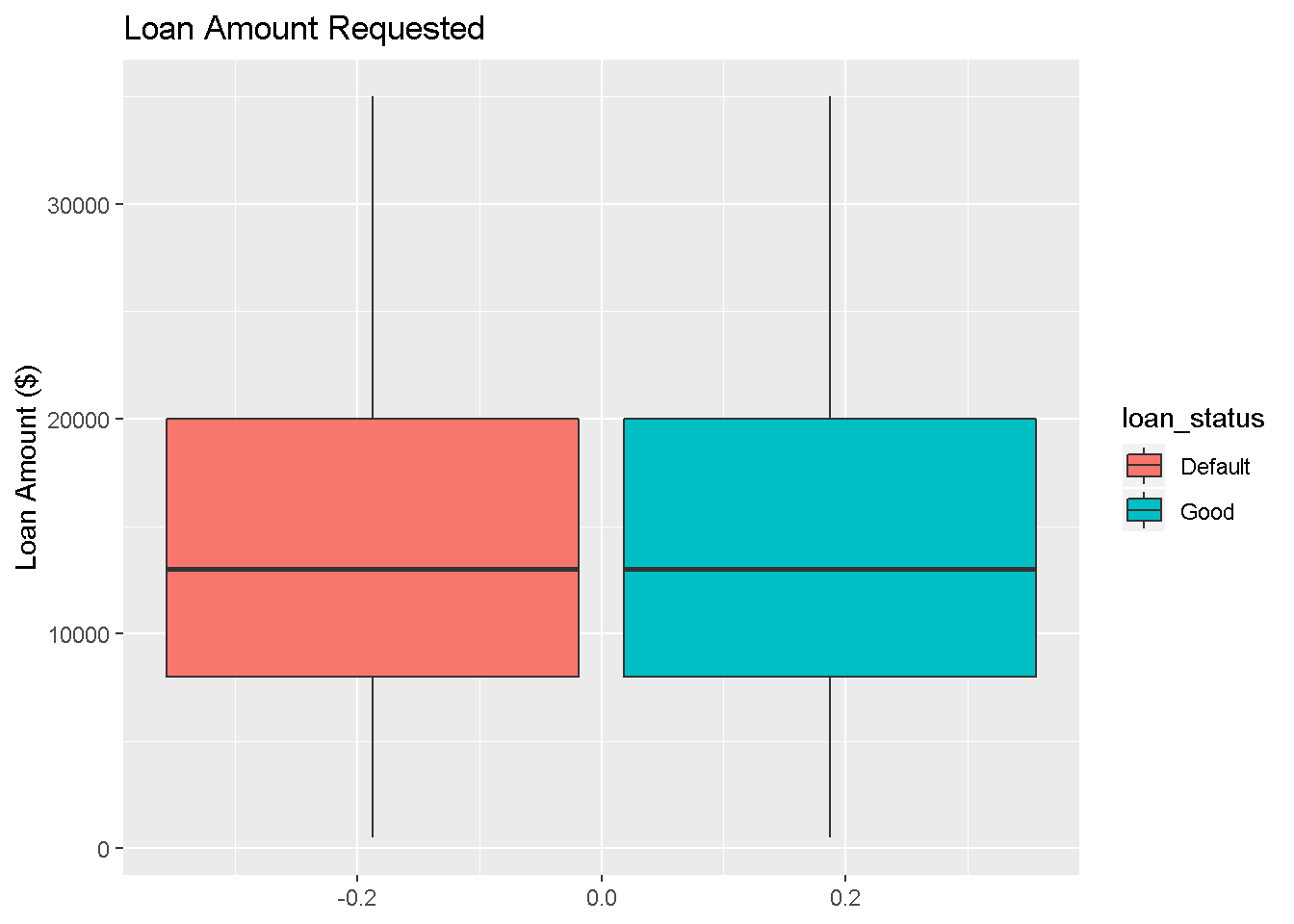 Another type of plot which can qualitatively show the correlation between the explanatory variables and factor response variable is the scatter plot. The below plot doesn’t seem to show the strong association seen in the boxplots for the two variables indicated.
#set.seed(12)
ggplot(df_new %>%
sample_frac(0.1) %>%
filter(score_days_interval>0.0))+
geom_point(aes(x=score_days_interval,y = int_rate,color=loan_status))+
labs(x="Days Elapsed",y="Interest Rate %", title = "Loan Status binary variable segregation scatter plot")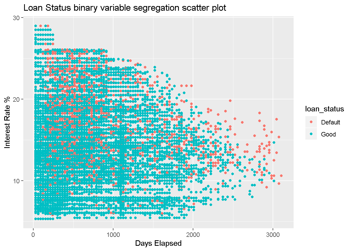 Installment amount doesn’t show strong correlation with the loan status.
ggplot(df_new,aes(y=installment,fill=loan_status))+
geom_boxplot()+
labs(y='Installment Amount ($)')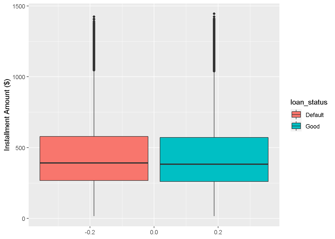 Since the dataset has a few categorical variables it makes sense to visualize some of the association. Barplots are one way to visualize this. Contingency tables are another way.
The following are the categorical/ordinal variables in the dataset.
df_new %>%
select_if(negate(is.numeric)) %>%
colnames()## [1] "term" "grade" "emp_length"
## [4] "home_ownership" "verification_status" "loan_status"
## [7] "purpose"The below barplot shows the absolute counts of Loan Tern split by loan default status. There seems to be no clear indication of association between the two variables.
df_new %>%
select(term,loan_status) %>%
ggplot(aes(x=term,fill=loan_status)) + geom_bar(position=position_dodge()) +
labs(x= "Loan Term",title = "Term of the Loan")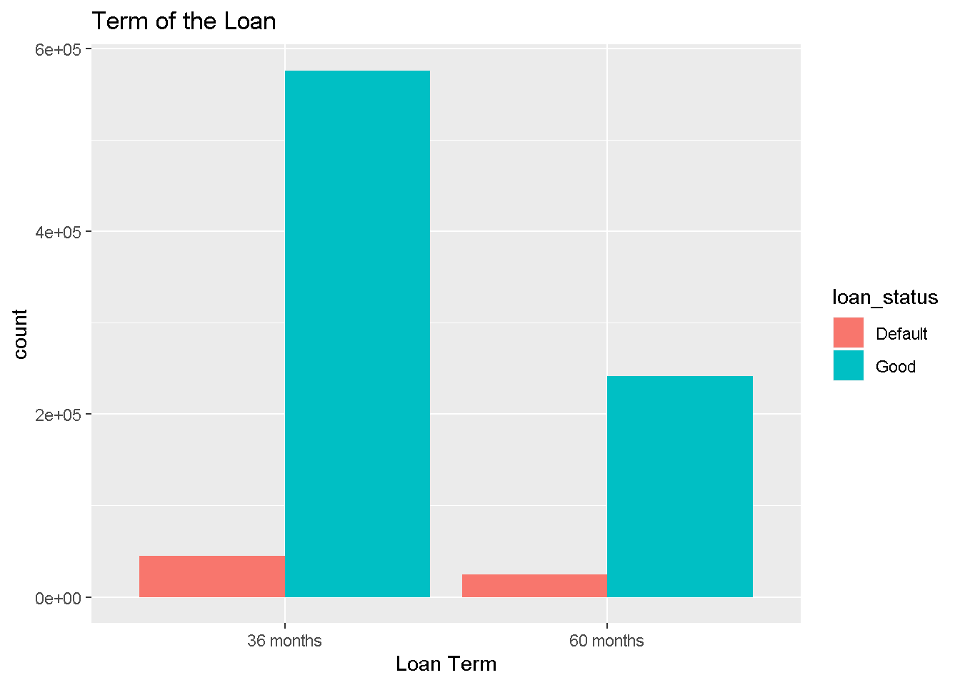 Following along the samelines,
df_new %>%
select(grade,loan_status) %>%
ggplot(aes(x=grade,fill=loan_status)) + geom_bar(position=position_dodge()) +
labs(x= "Grade",title = "Loan Grade")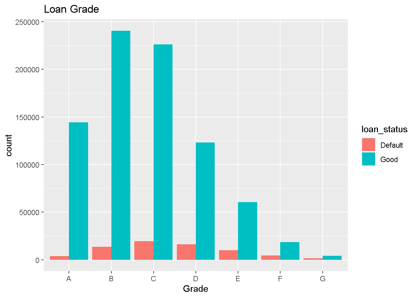
ggplot(df_new %>%
select(c(emp_length,loan_status)) %>%
na.omit(),
aes(x=emp_length,fill=loan_status))+
geom_bar(position=position_dodge())+
labs(x= "Employment Length",title = "Association between Employment Length and Loan Status")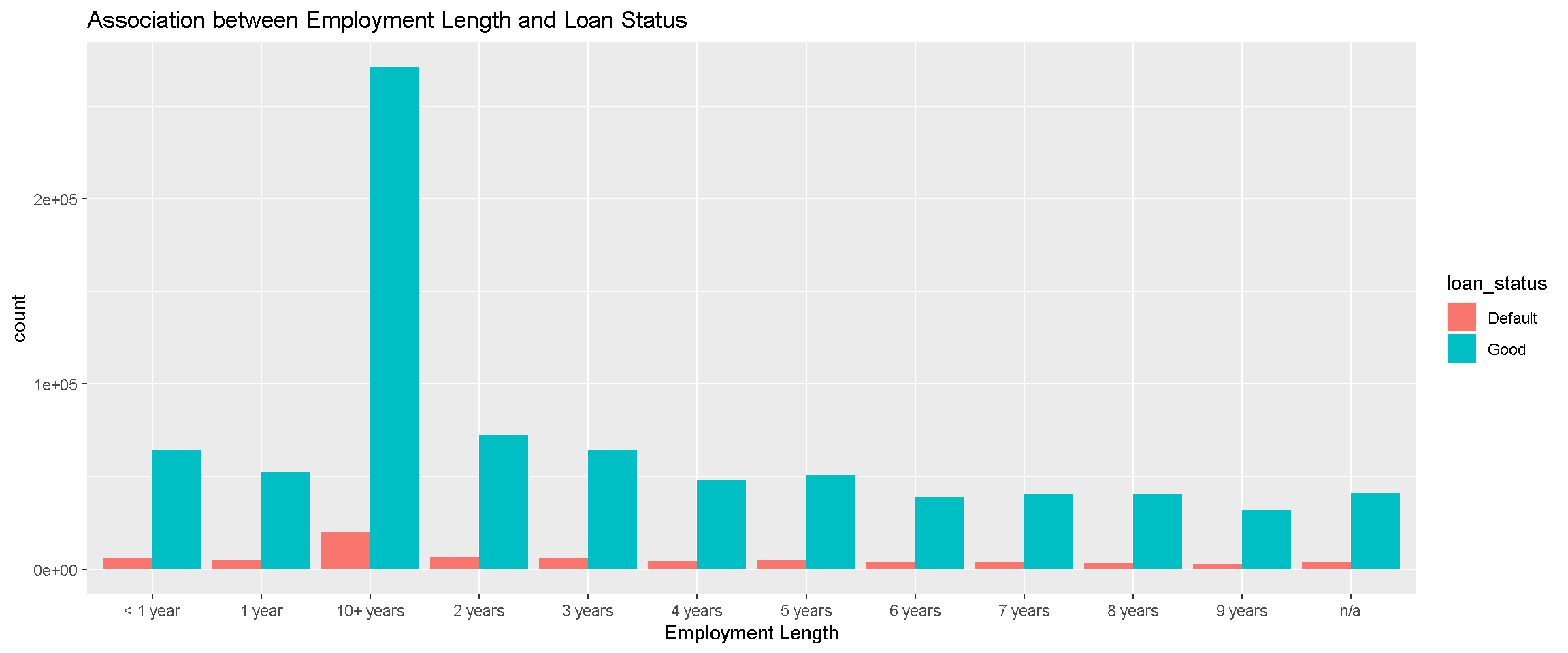 It is not clear whether Employment length is associated with Loan status from the above plot. The data can be transformed in the following way to visualize this association better. % Defaulted (percent defaulted for each employment length). There seems to be no clear association between the employment length and loan status. Empolyment length can be considered as an ordinal variable with < 1 year being the smallest and 10+ years being the largest on the scale.
emp_status_full <- df_new %>%
select(emp_length,loan_status) %>%
group_by(emp_length,loan_status) %>%
summarise(count = n())
emp_status_full %>%
group_by(emp_length) %>%
summarise(total = sum(count))## # A tibble: 12 x 2
## emp_length total
## <fct> <int>
## 1 < 1 year 70497
## 2 1 year 57028
## 3 10+ years 291339
## 4 2 years 78796
## 5 3 years 69971
## 6 4 years 52491
## 7 5 years 55660
## 8 6 years 42908
## 9 7 years 44556
## 10 8 years 43923
## 11 9 years 34624
## 12 n/a 44803emp_status_full %>%
filter(loan_status == "Default")%>%
inner_join(
emp_status_full %>%
group_by(emp_length) %>%
summarise(total = sum(count)),by='emp_length'
) %>%
mutate(percent_defaulted = 100*count/total) %>%
ggplot(aes(x=emp_length,y=percent_defaulted)) +
geom_point(color='dark red')+
labs(x="Employment Length",y="% Defaulted",title = "% Defaulted vs Employment Length")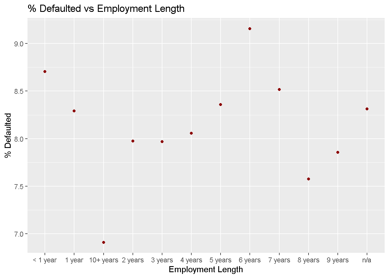
df_new %>%
select(home_ownership,loan_status) %>%
ggplot(aes(x=home_ownership,fill=loan_status)) + geom_bar(position=position_dodge()) +
labs(x= "Home Ownership",title = "Loan Grade")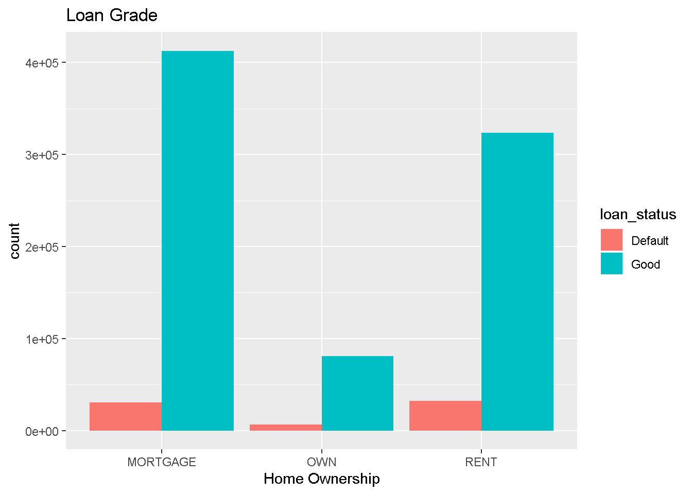
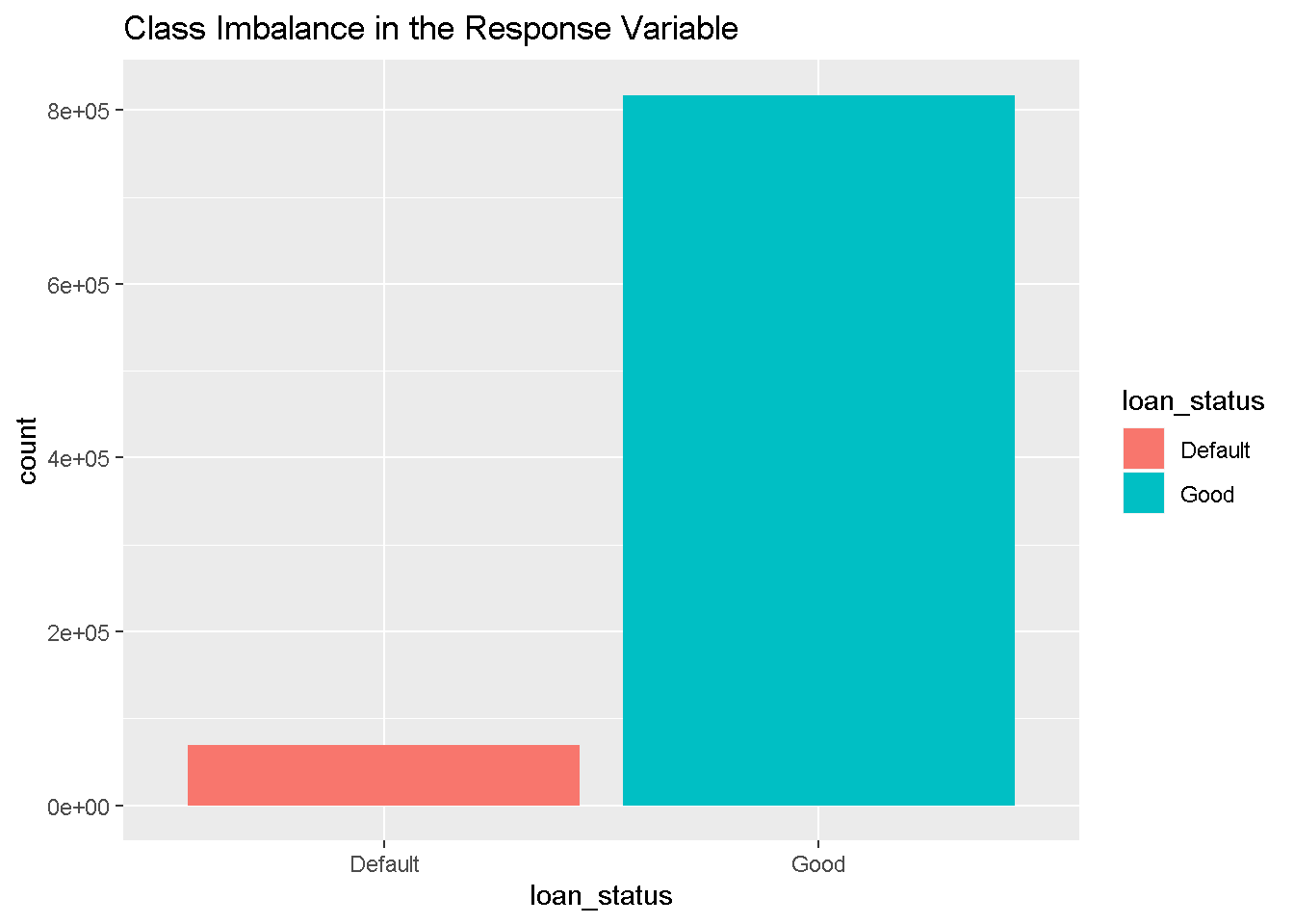
Finally the loan status response variable is highly imbalanced as shown below. Hence the performance of any classification algorithm should be evaluated using the area under the ROC curve.
ggplot(df_new,aes(x = loan_status,fill=loan_status)) +
geom_bar() +
labs(title = 'Class Imbalance in the Response Variable')